If you try plugging LeJEPA’s SIGReg loss [1] into standard text embeddings, your loss curve will likely flatline. I spent days debugging an implementation that stubbornly hovered around a loss of 5.0, refusing to learn. The fix? A single line of math.
The journey to that one-line fix started while I was working on a different paper, “Do Reasoning Models Enhance Embedding Models?”. I was measuring the isotropy of Qwen3-Embedding-8B [2] and stumbled upon something surprising: despite being trained on nearly 200M samples, its embedding space was highly anisotropic.
In theory, contrastive learning (like InfoNCE) is supposed to optimize both alignment and uniformity [3]. Positive pairs should pull together, while everything else spreads evenly across the hypersphere.
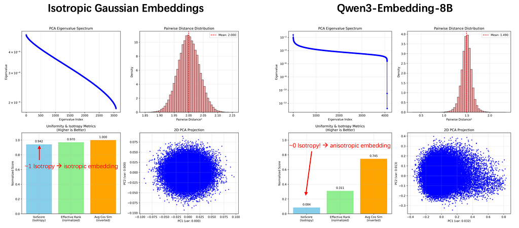
By isotropy, I mean that the embedding distribution uses its dimensions evenly instead of concentrating most of its variance in a small number of directions. A perfectly isotropic representation has no privileged axis. I measured this using IsoScore, which summarizes this variance distribution. Higher means closer to isotropic; near-zero indicates strong anisotropy.
Take a look at Figure 1: the left side shows a beautiful, isotropic Gaussian distribution. The right side shows the highly anisotropic reality of Qwen3-Embedding-8B. Text embeddings don’t have to look literally Gaussian in every detail, but the stark contrast in the figure makes the geometry problem visually obvious.
This anisotropy issue led me back to LeJEPA (Balestriero and LeCun). One detail I love about their work is that isotropy is not treated as a heuristic afterthought. They use SIGReg (Sketched Isotropic Gaussian Regularization) to explicitly constrain learned representations toward an isotropic Gaussian distribution.
The core idea is elegant. Instead of comparing full high-dimensional distributions — which is expensive — SIGReg basically projects embeddings onto many random unit directions and checks whether each one-dimensional projection looks like 𝒩(0, 1):

where 𝒜 is a set of random unit vectors and T is the Epps–Pulley
statistic, which is a scalar test of how Gaussian a sample looks, evaluated through its empirical characteristic function (ECF).
The key insight: if projections along every random direction look Gaussian with variance 1, then the full distribution must be (approximately) isotropic Gaussian. Linear complexity, no covariance matrix needed.
In LeJEPA, SIGReg is applied to unnormalized embeddings. But in text embedding training, InfoNCE almost always operates on L₂-normalized embeddings.
Let u ∈ ℝᴰ be an L₂-normalized embedding where |u|₂ = 1, and let a ∈ ℝᴰ be a random unit projection direction. The 1D projection is X = u ⋅ a = ∑ᵢ₌₁ᴰ uᵢ aᵢ.
Setup: Assume u is drawn from an isotropic distribution on Sᴰ⁻¹ (the ideal, collapse-free case). By symmetry, the same result holds for fixed u with random a.

by the symmetry of the uniform distribution on Sᴰ⁻¹. For the second moment, expand the square:

For uniform a on Sᴰ⁻¹, the cross terms vanish by symmetry: E[aᵢ aⱼ] = 0 for i ≠ j. For the diagonal terms, since all coordinates are exchangeable (i.e., E[a₁²]=E[a₂²]=⋯=E[a_D²]), and |a|² = ∑ᵢ aᵢ² = 1:

Therefore:

And since E[X] = 0:

First we briefly explain why we care E[cos(t ⋅ X)]. Since SIGReg relies on the Characteristic Function (CF), which is essentially the Fourier transform of a probability distribution. For a random variable X:

Where i is the imaginary unit and t is a frequency parameter. Using Euler’s formula, we can expand this into real and imaginary parts:

For a standard Gaussian G∼𝒩(0, 1),

Because 𝒩(0, 1) is symmetric around zero,

so the Gaussian target is entirely captured by:

Now we prove that E[cos(t ⋅ X)] ≈ 1 for all t ∈ [0, 3] when D is large.
Proof: Expand cos in a Taylor series and use the moments derived above. For a uniform sphere distribution, the higher moments of X are:

where (2k−1)!! = 1 ⋅ 3 ⋅ 5 ⋯ (2k−1). Using the Taylor expansion of cos:

The first three terms are (the rest are O(D⁻³)):

Numerically at t = 3 and D = 768:

Note that SIGReg is trying to compare the projection against 𝒩(0,1), which has a characteristic function of ϕ(t) = exp(−t²/2). Therefore for t=3, ϕ(t=3) = exp(−9/2) ≈ 0.0111.

This is near the maximum possible value of 1. Even if your embedding space is perfectly isotropic, it looks completely wrong to SIGReg. Very weird.
The gradient of the loss with respect to embedding uᵢ (for the cosine term at one slice a, one knot t):

To minimize the loss, the optimizer applies a negative gradient step, pushing uᵢ in the direction that increases sin(t, uᵢ ⋅ a) (positive values), i.e., increasing |uᵢ ⋅ a|.
On the unit sphere, a larger projection magnitude can only be achieved by concentrating the embeddings along a few directions, i.e., anisotropy. The loss is inadvertently rewarding collapse.
The solution is incredibly simple. Before applying SIGReg, just multiply the normalized embedding by √D:

Using the exact moments of X’ = √D ⋅ Z₁ (where Z₁ is the first coordinate of a uniform sphere vector), with extra Dᵏ in the nominator that comes from the √D:

Let’s verify it on some moments of X’. For k=2 (fourth moment):

For k=3 (sixth moment):

All moments converge to those of 𝒩(0,1) with relative error O(k/D). The CF:

Compared to the standard Gaussian CF:

Now look at the difference at t = 3 and D = 768:

So the residual CF error for a perfectly isotropic sphere distribution is ≈ 0.026 at t = 3, compared to ≈ 0.98 before the √D scaling fix, which is a 37× improvement.
More importantly, the sign of the gradient is now correct: if embeddings collapse (ECF approaches a constant oscillation, deviating far from exp(-t²/2)), the loss grows, and the gradient pushes back toward spreading. Simple enough, right?
Here is how you can implement this practically in PyTorch:
import mathimport torch
import torch.nn.functionalas F

def sigreg_loss(
    embeddings: torch.Tensor,
    num_directions:int =16,
    num_knots:int =16,
    t_max:float =3.0,) -> torch.Tensor:
    """
    SIGReg for L2-normalized text embeddings.
    The key step is scaling normalized embeddings by sqrt(D) before
    matching random 1D projections to N(0, 1).
    """
    batch_size, dim = embeddings.shape
    # InfoNCE usually works with normalized embeddings.
    z = F.normalize(embeddings, p=2, dim=-1)

    # THE FIX: SIGReg expects unit-variance random projections.
    z = z * math.sqrt(dim)

    directions = torch.randn(num_directions, dim, device=z.device, dtype=z.dtype)
    directions = F.normalize(directions, p=2, dim=-1)
    projections = z @ directions.T

    knots = torch.linspace(0.0, t_max, num_knots, device=z.device, dtype=z.dtype)
    tx = projections.unsqueeze(-1) * knots
    ecf_real = torch.cos(tx).mean(dim=0)
    ecf_imag = torch.sin(tx).mean(dim=0)

    target_real = torch.exp(-0.5 * knots.square()).unsqueeze(0)
    target_imag = torch.zeros_like(target_real)
    loss = (ecf_real - target_real).square() + (ecf_imag - target_imag).square()

    return loss.mean()
You can also find our implementation in https://github.com/lucaswychan/gritlm-re (specifically, gritlm/training/model.py).
Empirically, using Qwen2.5–0.5B as the backbone, this tweaked SIGReg noticeably improves isotropy. While there is a slight tradeoff with MTEB performance, the most encouraging result is batch size efficiency.
Take a look at Figure 2, where we set up a head-to-head comparison between two models:
(For context, we used the exact same training recipe from the paper, “Do Reasoning Models Enhance Embedding Models?” , where you can find all the training details in Appendix A).
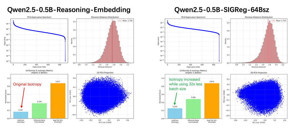
Here is the crazy part. As you can see in the chart, standard contrastive learning normally forces you to brute-force your way out of representation collapse by using massive, memory-hogging batch sizes. The baseline model relied on a hefty batch size of 2048 just to maintain uniformity.
But with our scaled SIGReg explicitly steering the distribution toward isotropy? I slashed the batch size all the way down to 64 and still achieved a more isotropic space.
By multiplying by √D and letting SIGReg do its job, huge batch sizes are no longer a strict requirement. Instead of using a giant batch as an expensive band-aid for model collapse, the regularizer attacks the root problem directly.
SIGReg and InfoNCE are a great match — you just have to respect the geometry.
Of course, no method is completely bulletproof, and there are a couple of limitations to this approach:

Figuring out how SIGReg behaves at scale, and closing that MTEB gap , is strictly future work. Or, knowing me, probably the subject of my next paper.
[1] Balestriero, R., & LeCun, Y. (2025). Lejepa: Provable and scalable self-supervised learning without the heuristics. arXiv preprint arXiv:2511.08544.
[2] Zhang, Y., Li, M., Long, D., Zhang, X., Lin, H., Yang, B., … & Zhou, J. (2025). Qwen3 embedding: Advancing text embedding and reranking through foundation models. arXiv preprint arXiv:2506.05176.
[3] Wang, T., & Isola, P. (2020, November). Understanding contrastive representation learning through alignment and uniformity on the hypersphere. In International conference on machine learning (pp. 9929–9939). PMLR.
[4] Enevoldsen, K.C., Chung, I., Kerboua, I., Kardos, M., Mathur, A., Stap, D., Gala, J., Siblini, W., Krzemi’nski, D., Winata, G.I., Sturua, S., Utpala, S., Ciancone, M., Schaeffer, M., Sequeira, G., Misra, D., Dhakal, S., Rystrøm, J., Solomatin, R.S., cCaugatan, O.V., Kundu, A., Bernstorff, M., Xiao, S., Sukhlecha, A., Pahwa, B., Poswiata, R., Kranthikiran, G., Ashraf, S., Auras, D., Pluster, B., Harries, J.P., Magne, L., Mohr, I., Hendriksen, M., Zhu, D., Gisserot-Boukhlef, H., Aarsen, T., Kostkan, J., Wojtasik, K., Lee, T., vSuppa, M., Zhang, C., Rocca, R., Hamdy, M., Michail, A., Yang, J., Faysse, M., Vatolin, A., Thakur, N., Dey, M., Vasani, D., Chitale, P.A., Tedeschi, S., Tai, N., Snegirev, A., Gunther, M., Xia, M., Shi, W., Lù, X., Clive, J., Krishnakumar, G., Maksimova, A.D., Wehrli, S., Tikhonova, M., Panchal, H.S., Abramov, A., Ostendorff, M., Liu, Z., Clematide, S., Miranda, L.V., Fenogenova, A., Song, G., Safi, R.B., Li, W., Borghini, A., Cassano, F., Su, H., Lin, J., Yen, H., Hansen, L., Hooker, S., Xiao, C., Adlakha, V., Weller, O., Reddy, S., & Muennighoff, N. (2025). MMTEB: Massive Multilingual Text Embedding Benchmark. ArXiv, abs/2502.13595.